Fast Generation of Non-Uniform Random Numbers

Suppose you want to chose between several values randomly with uniform probability. That is, you might have 5 options, A, B, C, D, E. You want to chose among them with equal probability. You generate a random number from [0-1), and multiply that number by 5, round down to the nearest integer, use that to index into an array of letters.

But what if you want to chose among these values with non-uniform probability? Suppose for each symbol you assign a likelihood, and you want to generate symbols from a non-uniform probability distribution:

   A: 0.05
   B: 0.10
   C: 0.10
   D: 0.20
   E: 0.55

It is possible to do this, in constant time, and with memory that scales linearly with the number of symbols: decompose the probabilities of each N symbols into N-1 binary distributions.

Some Naive Methods

Table Method: An obvious method of doing this would be to create a table that is in proportion to the probabilities, and select uniformly from the elements in the table:

   A, B, B, C, C, D, D, D, D, E, E, E, E, E, E, E, E, E, E, E

This will generate the symbols in constant time, but the table can become very large if the probabilities are very uneven. In this case the least common factor is 0.05, so you need a table with 20 elements. If the least common factor had been say 0.0001, you would need a table with 10000 elements.

The other problem with this method is that if you change the probability of any symbol, you would have to regenerate the entire table.

In C, this method is sometimes implemented with a giant “switch” statement. It works in constant time, but in this case you still have a table, it is just expressed in code rather than in data.

Cumulative probability Methods: You create a table of cumulative probabilities:

   A: 0.05
   B: 0.15
   C: 0.25
   D: 0.45
   E: 1.00

Then generate a number from [0-1), and then test that number for each of the given ranges. E.g. if N smaller than 0.05 return A, if smaller than 0.15 return B etc.

This method will generate numbers in time that scales linearly with the the number of elements in the distribution.

An improvement on this method is to use a binary search to find the desired symbol. This will scale as O=log(n). A lot better – but not constant time.

Decomposing Non-Uniform Distributions

A better way is to convert the input set of probabilities into a set of binary distributions.

Any discrete non-uniform probability distribution can be decomposed into N-1 non-uniform binary distributions. For example, consider this distribution:

   A: 0.05
   B: 0.10
   C: 0.10
   D: 0.20
   E: 0.55

It can be expressed as:

   1. A/E: 0.20/0.80
   2. B/E: 0.40/0.60
   3. C/E: 0.40/0.60
   4. D/E: 0.80/0.20

To generate a number: first chose a distribution using a uniform generator, and then chose between the first or second symbol according to the binary probability.

For example, assume you have a uniform random number generator that generates values in the range of [0-1).

First you would generate a random number, multiply by the number of distributions, 4, and round down to get a number from [0-3], say 2, selecting the binary distribution for B/E. Then generate another number from [0-1), and chose between the first or second symbol according to the probability. In this case if the number is smaller or equal 0.40 generate B, otherwise generate E.

To verify the decomposed binary distributions: divide each probability by the number of distributions and confirm that they sum to the original non-decomposed probabilities:

   1. A/E: 0.20/4 = 0.05, 0.80/4 = 0.20
   2. B/E: 0.40/4 = 0.10, 0.60/4 = 0.15
   3. C/E: 0.40/4 = 0.20, 0.60/4 = 0.15
   2. D/E: 0.80/4 = 0.20, 0.20/4 = 0.05

Now summing the probabilities for each symbol:

   A: 0.05 ( from 1 )
   B: 0.10 ( from 2 )
   C: 0.20 ( from 3 )
   D: 0.20 ( from 4 )
   E: 0.55 ( from 1-4: 0.20 + 0.15 + 0.15 + 0.05 = 0.55 )

Decomposing Non-Uniform Distributions into Binary Distributions

Step 1: Determine the number of binary distributions.

We said earlier that any non-uniform probability distribution of N symbols can be decomposed into N-1 binary distributions. But you can actually do a little better than that – you can ignore all symbols with probability zero. So the first thing we do is count up the number of symbols with a non-zero probability, and use that to determine the number of binary distributions.

Step 2: Compute the probability of choosing any of binary distribution.

If the number of distributions is N, then this probability is just 1/N. This is the portion of the probability space that each distribution will account for. For example with 5 distributions, each distribution has a probability of 0.20. Each one must account for 1/5 of the probability space. That is, each distribution will represent one portion of the probability of each of two symbols, such that the sum of the probability of each is equal to the probability of choosing that distribution.

Step 3: Generate the binary distributions.

For each distribution we chose 2 symbols: one which has a probability A, which smaller than or equal to 1/N, and another which has a probability B, greater than or equal to ((1/N) – A).

We create the new distribution by setting its two symbols, and setting its probability to ( N * A ).

As we create new binary distributions, we subtract the probabilities in our input non-uniform distribution to account for each generated binary distribution, until all the input probabilities are zero.

Decomposing a Non-Uniform Distribution: Example

Before we get to the code lets run through an example, given the following input probability distribution:

   A: 0.28
   B: 0.20
   C: 0.05
   D: 0.00
   E: 0.12
   F: 0.35

We have 5 non-zero probabilities, so we need to generate 4 binary distributions. The probability of each distribution is 1/4, or 0.25. Since the probability of D is zero, we can safely ignore it.

To generate the first probability we consider each symbol in turn. A has a probability larger than 0.25, so we skip it. B has a probability 0.20, so we chose that as the first symbol of our first distribution.

We compute the minimum probability for the second symbol in the first distribution:

0.25 - 0.20 = 0.05

A has a probability greater than 0.05, so we chose A for the second symbol in the first distribution.

We compute the probability of choosing B vs. A in the first distribution:

4 * 0.20 = 0.80

The first distribution is therefore:

B/A: 0.80/0.20

We now adjust the input non-uniform distribution. We set B to zero and therefore remove it, and we subtract ( 0.25 – 0.20 ), or 0.05, from the probability of A:

   A: 0.23
   C: 0.05
   E: 0.12
   F: 0.35

We repeat this process three times for each remaining binary distributions.

So for the second distribution, A now has a probability smaller than 0.25. 0.25 – 0.23 = 0.02. Now we choose a symbol with probability greater than 0.02, so we choose C. Therefore we now have the following two binary distributions:

B/A: 0.80/0.20
A/C: 0.92/0.08

The input distribution is now:

   C: 0.03
   E: 0.12
   F: 0.35

For the second distribution C has a probability smaller than 0.25. 0.25 – 0.03 = 0.22. Choose a symbol with probability greater than 0.22, so we choose F. Now we have the following three binary distributions:

B/A: 0.80/0.20
A/C: 0.92/0.08
C/F: 0.12/0.88

And the input distribution is now:

   E: 0.12
   F: 0.13

We have two symbols remaining. Note that their probabilities sum to 0.25, so at the end of this step the input distribution will be completely accounted for.

We create the last distribution from the remaining two symbols:

B/A: 0.80/0.20
A/C: 0.92/0.08
C/F: 0.12/0.88
E/F: 0.48/0.52

We can verify the binary distributions. Divide each probability by the number distributions:

   1. B/A: 0.80/4 = 0.20, 0.20/4 = 0.05
   2. A/C: 0.92/4 = 0.23, 0.08/4 = 0.02
   3. C/F: 0.12/4 = 0.03, 0.88/4 = 0.22
   4. E/F: 0.48/4 = 0.12, 0.52/4 = 0.13

And sum the resulting probabilities for each symbol:

A = 0.23 + 0.5  = 0.28 ( from 1 and 2 )
B               = 0.20 ( from 1 )
C = 0.02 + 0.03 = 0.05 ( from 2 and 3 )
D               = 0.00
E               = 0.12 ( from 4 )
F = 0.22 + 0.13 = 0.35 ( from 3 and 4 )

Implementation

Now that we have the theory in place we can go over the code.

First we’ll go over the code to represent binary distributions and to generate non-uniform symbols numbers using them. All the code is pretty easy. Decomposing into binary distributions is the most complex part, so we’ll go over that at the end.

A Uniform Random Number Generator

First lets implement a simple uniform random number generator. We will use this to build our non-uniform generator.

   #define U32_MAX 0xFFFFFFFF

   class KxuRand
   {
   public:
      virtual ~KxuRand() { ; }
      virtual u32    getRandom() = 0;
      virtual double getRandomUnit() { return (((double)getRandom()) / U32_MAX ); }
   };

   class KxuRandUniform : public KxuRand
   {
   public:
      virtual ~KxuRandUniform() { ; }
      virtual void setSeed( u32 seed ) = 0;

      u32  getRandomInRange( u32 n ) 
         { u64 v = getRandom(); v *= n; return u32( v >> 32 ); }
      u32  getRandomInRange( u32 start, u32 end ) 
         { return getRandomInRange( end - start ) + start; }
  };

   // a dead simple Linear Congruent random number generator
   class KxuLCRand : public KxuRandUniform
   {
   public:
      KxuLCRand( u32 seed = 555 ) { setSeed( seed ); }
      void setSeed( u32 seed ) { if ( !seed ) seed = 0x333; mState = seed | 1; }
      u32 getRandom() { mState = ( mState * 69069 ) + 1; return mState; }

   private:
      u32 mState;
   };

KxuRand is a virtual base class for all our generators. From this we build a uniform generator, KxuRandUniform that will generate a random number from [0-N) with uniform probability – all values are equally probable.

I also include here a classic random number generator, the linear congruent generator, as KxuLCRand. This is a very fast and very simple generator with good performance. In practice, if you need high quality random numbers you should implement something like a mersenne twister, as a class derived from KxuRandomUniform

A Non-Uniform Random Generator

For efficiency and accuracy, we’re going to implement the non-uniform generator using 32-bit fixed point math, with all bits to the right of the decimal point ( aka 0.32 fixed point). Each integer will correspond to a number the range from [0-1).

You can convert btween 0.32 fixed point and floating point like this:

   double fixedToFloat_0_32( u32 val ) { return (((double)val) / U32_MAX ); }
   u32    floatToFixed_0_32( double val ) { return (u32)( val * U32_MAX ); }

Using fixed point math has a number of advantages:

1. Fixed point is generally faster than floating point.
2. The values we are going to use are all in the range of [0-1). Floating point numbers reserve some bits for the exponent, but in our case the exponent will always be the same, so by using 32 bit fixed point we actually have more resolution and therefore accuracy.

Now we implement a trivial class to represent a binary distribution:

   class Distribution
   { 
   public:
      Distribution() { ; }
      Distribution( u32 a, u32 b, u32 p ) { mA = a; mB = b, mProb = p; }

      u32 mA; 
      u32 mB; 
      u32 mProb; 
   };

This class just holds the two symbols in the distribution and a probability. The symbols, mA and mB are indexes into an array of your symbols. So if you literally wanted to generate letters like A, B, C, D, E, you create an array somewhere with those letters, and use the numbers generated by generator to index into this table.

Next we declare the interface for our non-uniform generator:

   class KxuNuRand : public KxuRand
   { 
   public:
      KxuNuRand( const KxVector<u32>& dist, KxuRandUniform* rand );
      u32 getRandom();

   protected:
      KxVector<Distribution> mDist;
      KxuRandUniform* mRand;
   };

KxVector is simple vector container similar to std::vector.

To initialize the generator you pass in an array of integers that are in proportion to the probabilities in your non-uniform distribution. When we initialize the system we will normalize these into a set of probabilities that sum to one. So all you need to do is pass in integer proportions.

If your input distribution is already represented as floating point values that sum to 1, you can multiply each probability by U32_MAX, and cast it to an unsigned int.

To represent our example distribution you could pass in:

   1, 2, 2, 4, 11

Or even:

   0.05 * U32_MAX, 
   0.10 * U32_MAX,
   0.20 * U32_MAX,
   0.20 * U32_MAX,
   0.55 * U32_MAX

Either way works, so long as the values are in the same proportions as your desired probabilities.

To generate a symbol:

   u32 KxuNuRand::getRandom()
   { 
      const Distribution& dist = mDist[mRand->getRandomInRange( mDist.size() )]; 
      return ( mRand->getRandom() <= dist.mProb ) ? dist.mA : dist.mB; 
   }

Decomposing a Non-Uniform Distribution

// Since we are using fixed point math, we first implement 
// a fixed 0.32 point inversion:  1/(n-1) 
#define DIST_INV( n ) ( 0xFFFFFFFF/( (n) - 1 ))

KxuNuRand::KxuNuRand( const KxVector<u32>& dist, KxuRandUniform* rand )
{
   mRand = rand;

   if ( dist.size() == 1 )
   {
      // handle a the special case of just one symbol.
      mDist.insert( Distribution( 0, 0, 0 ));

   } else {
      
      // The non-uniform distribution is passed in as an argument to the
      // constructor. This is a series of integers in the desired proportions.
      // Normalize these into a series of probabilities that sum to 1, expressed 
      // in 0.32 fixed point.
      KxVector<u32> p; p = dist;
      normProbs( p );
      
      // Then we count up the number of non-zero probabilities so that we can 
      // figure out the number of distributions we need.
      u32 numDistros = 0;
      for ( u32 i = 0; i < p.size(); i++ )
         if ( p[i] ) numDistros++;
      if ( numDistros < 2 ) numDistros = 2;
      u32 thresh = DIST_INV( numDistros );

      // reserve space for the distributions.      
      mDist.resize( numDistros - 1 );
      
      u32 aIdx = 0; 
      u32 bIdx = 0; 
      for ( u32 i = 0; i < mDist.size(); i++ ) 
      { 
         // find a small prob, non-zero preferred
         while ( aIdx < p.size()-1 )
         {
            if (( p[aIdx] < thresh ) && p[aIdx] ) break;
            aIdx++;
         }
         if ( p[aIdx] >= thresh )
         {
            aIdx = 0;
            while ( aIdx < p.size()-1 )
            {
               if ( p[aIdx] < thresh ) break;
               aIdx++;
            }
         }
         
         // find a prob that is not aIdx, and the sum is more than thresh.
         while ( bIdx < p.size()-1 )
         {
            if ( bIdx == aIdx ) { bIdx++; continue; } // can't be aIdx
            if ((( p[aIdx] >> 1 ) + ( p[bIdx] >> 1 )) >= ( thresh >> 1 )) break;
            bIdx++; // find a sum big enough or equal
         }

         // We've selected 2 symbols, at indexes aIdx, and bIdx.
         // This function will initialize a new binary distribution, and make 
         // the appropriate adjustments to the input non-uniform distribution.
         computeBiDist( p, numDistros, mDist[i], aIdx, bIdx );

         if (( bIdx < aIdx ) && ( p[bIdx] < thresh ))
            aIdx = bIdx;
         else
            aIdx++;
      }       
   }
}

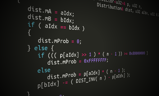
This is the function that creates a new binary distribution. We’ve already described the algorithm. The only wrinkle here is doing it in fixed point:

static void computeBiDist( KxVector<u32>& p, u32 n, 
                           Distribution& dist, u32 aIdx, u32 bIdx ) 
{ 
   dist.mA = aIdx; 
   dist.mB = bIdx; 
   if ( aIdx == bIdx )
   {
      dist.mProb = 0;
   } else {
      if ((( p[aIdx] >> 1 ) * ( n - 1 )) >= 0x80000000 )
         dist.mProb = 0xFFFFFFFF;
      else
         dist.mProb = p[aIdx] * ( n - 1 ); 
      p[bIdx] -= ( DIST_INV( n ) - p[aIdx] );
   }
   p[aIdx] = 0; 
} 

And finally this function normalizes a set of integer to create a set of probabilities that sum to 1, expressed in 0.32 fixed point:

static void normProbs( KxVector<u32>& probs )
{
   u32 scale = 0;
   u32 err = 0;
   u32 shift = 0;
   u32 max = 0;
   u32 maxIdx = 0;

   // how many non-zero probabilities?
   u32 numNonZero = 0;
   for ( u32 i = 0; i < probs.size(); i++ )
      if ( probs[i] ) numNonZero++;

   if ( numNonZero == 0 )
   {
      // degenerate all zero probability array. 
      // Can't do anything with it... result is undefined
      assert(0);
      return;
   }

   if ( numNonZero == 1 )
   {
      // trivial case with only one real prob - handle special because 
      // computation would overflow below anyway.
      for ( u32 i = 0; i < probs.size(); i++ )
         probs[i] = probs[i] ? U32_MAX : 0;
      return;
   }

   // figure out the scale
again:
   for ( u32 i = 0; i < probs.size(); i++ ) 
      scale += (( probs[i] << shift ) >> 8 );

   if (( scale < 0xFFFF ) && ( shift < 24 )) 
   {
      shift += 8;
      goto again;
   }

   assert( scale );
   
   scale = 0x10000000 / (( scale + 0x7FF ) >> 12 );

   // apply it
   for ( u32 i = 0; i < probs.size(); i++ ) 
   {
      probs[i] = ((( probs[i] << shift ) + 0x7FFF ) >> 16 ) * scale;
      err += probs[i];
      if ( probs[i] > max )
      {
         max = probs[i];
         maxIdx = i;
      }
   }

   // correct any accumulated error - it should be negligible. Add it  
   // to the largest probability where it will be least noticed.
   probs[maxIdx] -= err;
}

Some Performance Metrics

My friend Roger Gonzalez implemented a version of this algorithm in Javascript and produced some performance graphs comparing it to other methods.

The table shows simply that the binary distribution method does not slow down as the size of the distribution increases.

Resources:

Non-Uniform Distributions	Roger Gonzalez’ implementation of this algorithm in Javascript
Darts, Dice, and Coins: Sampling from a Discrete Distribution	Keith Schwartz’ detailed explanation and proofs for this algorithm and a java implementation
ransampl	Joachim Wuttke’s implementation of the alias method in c
Alias method	Wikipedia’s entry on the alias method
New fast method for generating discrete random numbers with arbitrary frequency distributions	A. J. Walker’s original 1974 paper on this method
An Efficient Method for Generating Discrete Random Variables with General Distributions	A. J. Walker’s 1977 paper on this method