Exponential Moving Averages for Irregular Time Series
In time series analysis there is often a need for smoothing functions that react quickly to changes in the signal. In the typical application, you may be processing an input signal in real time, and want to compute such things as the recent average value, or get an instantaneous slope for it. But real world signals are often noisy. A few noisy samples will make the current value of the signal, or its slope, vary widely.
Moving Averages
The simplest smoothing function is a windowed moving average. As samples come in you take an average of the most recent N values. This will smooth out spikes, but introduces a delay – or latency. Your average will always be delayed by the width of your moving average.
double movingAverage( double sample )
{
    static double buf[NUM_SAMPLES] = { 0 };
    static u32 idx = 0;
    buf[idx++] = sample;
    if ( idx >= NUM_SAMPLES ) idx = 0;

    double avg = 0;
    for ( u32 i = 0; i < NUM_SAMPLES; i++ )
       avg += buf[i];
    avg /= NUM_SAMPLES;

    return avg;
}
The example above is relatively expensive to compute. For each sample you have to iterate over the entire size of the window. But there are cheaper ways – keep the sum of all the samples in the window in a buffer, and adjust the sum as new samples come in:
double movingAverage( double sample )
{
    static double buf[NUM_SAMPLES] = { 0 };
    static u32 idx = 0;
    double sum = 0;

    sum -= buf[idx];
    sum += sample;
    buf[idx++] = sample;
    if ( idx >= NUM_SAMPLES ) idx = 0;

    return ( sum / NUM_SAMPLES );
}
Another type of moving average is the “weighted moving average” that weights for each position in the sample window. Before averaging you multiply each sample by the weight of that window position. Technically this is called a “convolution”.
One typical weighting function applies a bell curve to the sample window. This gives a signal which is more tuned to the center of the window, and still somewhat tolerant of noisy samples. In financial analysis you often use a weighting function that values recent samples more, to give a moving average that more closely tracks recent samples. Older samples are given progressively less weight. This somewhat mitigates the effects of latency, while still giving reasonably good smoothing:
double weightedMovingAverage( double sample, double* weights )
{
    static double buf[NUM_SAMPLES] = { 0 };
    static u32 idx = 0;
    buf[idx++] = sample;
    if ( idx >= NUM_SAMPLES ) idx = 0;

    double avg = 0;
    for ( u32 i = 0; i < NUM_SAMPLES; i++ )
       avg += buf[(idx + i ) % NUM_SAMPLES] * weights[i];
    avg /= NUM_SAMPLES;

    return avg;
}
With a weighted average, you always have to iterate over the entire window size for every sample ( unless you can constrain the allowed weights to certain functions).
The Exponential Moving Average
Another type of average is the exponential moving average, or EMA. This is often used where latency is critical, such as in real time financial analysis. In this average, the weights decrease exponentially. Each sample is valued some percent smaller than the next most recent sample. With this constraint you can compute the moving average very efficiently.
The formula is:
avgt = ( alpha * samplet ) + (( 1 – alpha ) * avgt-1 )
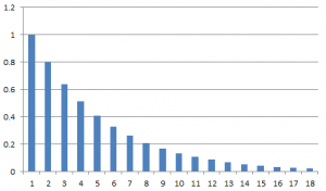
Where alpha is a constant that describes how the window weights decrease over time. For example if each sample was to be weighted at 80% of the value of the previous sample, you would set alpha = 0.2. The smaller alpha becomes the longer your moving average is. ( e.g. it becomes smoother, but less reactive to new samples ).
As you can see, for each new sample you only need to average it with the value of the previous average. So computation is very very fast.
In theory all previous samples contribute to the current average, but their contribution becomes exponentially smaller over time.
This is a very powerful technique, and probably the best if you want to get a moving average that responds quickly to new samples, has good smoothing properties and is fast to compute.
The code is trivial:
double exponentialMovingAverage( double sample, double alpha )
{
   static double cur = 0;
   cur = ( sample * alpha ) + (( 1-alpha) * cur );
   return cur;
}
EMA for Irregular Time Series
The standard EMA is fine when the signal is sampled at regular time intervals. But what if your samples come at irregular intervals?
Imagine a continuous signal which is sampled at irregular intervals. This is the usual situation in financial analysis. In theory there is a continuous function for the value of any financial instrument, but you only can sample this signal whenever someone actually executes a trade. So your data stream consists of a value, plus the time at which it was observed.
One way to deal with this is to convert the irregular signal to a regular signal, by interpolating between observations, and resampling. But this loses data, and it re-introduces latency.
It is possible to compute an EMA for an irregular time series directly:
double exponentialMovingAverageIrregular(
    double alpha, double sample, double prevSample,
    double deltaTime, double emaPrev )
{
   double a = deltaTime / alpha;
   double u = exp( a * -1 );
   double v = ( 1 - u ) / a;

   double emaNext = ( u * emaPrev ) + (( v - u ) * prevSample ) +
                    (( 1.0 - v ) * sample );
   return emaNext;
}
In this function, you pass in the current sample from your signal, and the previous sample, and the amount of time elapsed between the two, and the previous value returned by this function.
Results
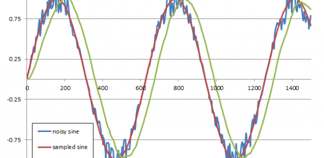
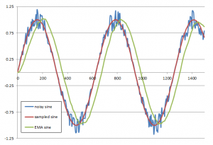
So how well does this work? To demonstrate I’ve generated a sine wave, then sampled it at irregular intervals, and introduced about 20% noise. That is the signal will vary randomly +- 20% from the original “true” sine signal.
How well does the irregular exponential moving average recover the signal?
The red line is the original sine wave – sampled at irregular intervals. The blue line is the signal with the noise added. The blue line is the only signal the EMA sees. The green line is the smoothed EMA. You can see it recovers the signal pretty well. A little wobbly, but what can you expect from such a noisy source signal?
It is shifted about 15% to the right, because the EMA does introduce some latency. The smoother you want it, the more latency you will see. But from this you can for example compute an instantaneous slope for a noisy irregular signal.
What can you do with that? Hmm….
Resources:
| Moving Average | A wikipedia page covering basic moving averages |
| A Framework for Analysis of Unevenly Spaced Time Series Data | Andreas Eckner’s paper on irregular time series analysis |
| Algorithms for Unevenly Space Time Series | Another Eckner paper on irregular time series. |
| Methods for Analysis of Financial Markets | Ulrich Muller’s method for irregular time series analysis. His academic papers are disappearing, but the method is still described in his patents. |
| Filtering of High Frequency Time Series Data | Another of Muller’s patents that describes among other things a method for irregular time series analysis. |
| Efficient Estimation of the Parameter Path in Unstable Time Series | One of Ulrich Muller’s papers on irregular time series analysis. |


Hey guy,
nice work, it’s exactly that what I need. But do you really tested the code on the website ?
It should be
double a = deltaTime / alpha;
then the algorithm works as supposed.
Thanks,
krater
Thanks for your comment… but unless I misunderstand you, the edit you suggest is the way the code is already.
Hi rafael, really nice post. I stumbled on your website by accident and it’s as if you’re posting exactly on the things I’m interested!
On the method now: Do you have some reference on the mathematical background of the “EMA for an irregular time series”? I’d love to understand a bit better how/why it works.
Thanks,
Petros
Hi
This is a great rundown of exponential moving averages of irregular spaced time series.
One question: How would you decide on the value of alpha. Usually you would use 2/(n+1) but if the time series is irregular. Problem here is what to decide is the value of n. In the case of time series this could tend to change the time period the ema is sample over quite dramatically.
Do you have any ideas?,
Thank you for this post!
Could you recommend any algorithm for counting number of irregular samples per last XX seconds?
Shouldn’t it be:
double a = deltaTime / (1 – alpha);
Otherwise it seems to reverse the weighting compared to the standard formula:
Large alpha => small a => large u => bigger weighting to emaPrev
Do you have any further info on the derivation of the formula?
Alright, vina24hmb caught my eye. Mobile experience is smooth, no lag. Content’s solid. I’d give it a thumbs up for usability. Give it a go: vina24hmb