Fast Approximate Distance Functions
The formula for the euclidean distance between two points, in three dimensions is:
d = (X2 + Y2 + Z2)1/2
In two dimensions its:
d = (X2 + Y2)1/2
Computing this function requires a square root, which even on modern computers is expensive.note It is solved by iterative approximation – which means the computer enters a loop approximating the square root until it is within a given error margin. If you are working on more limited hardware which does not have a square root function implemented in hardware, then computing even a small number of square roots may be prohibitive.

For many computations it is possible to compare square distances and so to avoid doing square roots at all. For example, if your computation is concerned only with comparing distances, then comparing square distances is equivalent. However, there are computations where you really do need to get distances – say if you need to normalize vectors, or you are implementing a collision system using spherical bounding volumes.
In these cases, if you cannot afford to compute the standard distance function, there are classes of functions which give a pretty good approximation to the distance function and which are composed entirely of easy to compute linear pieces. In theory you can keep making a linear approximation of a non-linear function arbitrarily accurate by adding more pieces. In fact this is not unlike what the square root function does when implemented on computers. The functions I will be discussing can generally approximate the distance within 2.5% average error, and with about a 5% maximum error with a small number of linear components and are therefore very fast to run. They can be adjusted to trade off maximum error for average error and you can construct functions that will move the error to certain places.
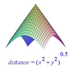
First lets look at a 3d plot of the true distance function. This 3d patch represents a euclidean distance function where x and y range from -1 to 1. The height of the plot represents the negative distance. So when x and y are equal to zero, the distance is equal to zero, and that is the peak of the cone. Increasing values of x and y correspond to points lower down on the cone. The cross section of this plot would look like a circle.
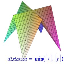
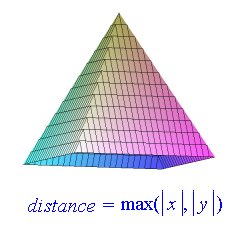
Here are plots of the maximum and minimum of the absolute value of x and y, where x and y range from -1 to 1. The maximum plot is a 4 sided pyramid. The point where x and y are equal to zero corresponds to the top of the pyramid. Its cross section is a square. You can see that the plot for the minimum tends to operate as an inverse of the pyramid. Its cross section looks like a cross.
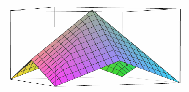
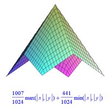
Therefore if you make a linear combination of these two functions you get a pretty good approximation to the distance function. Different scaling values for min and max will give you approximations with different properties. This one is balanced to produce the smallest possible maximum error. You can also balance the function to produce a minimum average error, or minimum average square error. You can see that the places of maximum error are where either x or y approach zero. That is, these are the places where the shape of the cross section tends to deviate most from the ideal circle. ( It is possible to reduce the error at these points to zero by adjusting the scaling factors, but at great cost to accuracy everywhere else ).
You can improve the accuracy of this function by adding a term specifically designed to correct error at these points. In this case we change the scaling of this function only where the larger of x or y, is greater than 16 times the value of the smaller of x or y. You can see in the plot of this new function that the sharp indentations where x or y approach zero are somewhat rounded out. You can continue to process further reducing the amount of error until it is suitably accurate for your purposes. Of course as you add linear pieces to the function it becomes more expensive to compute.
It is easy to demonstrate that for any approximate distance function that you want to work with the minimum and maximums of the absolute values of x and y. Consider that for the true distance function, for any given distance X you get points on a circle with radius X. So you are essentially trying to make an approximation of a circular graph using straight lines. Notice that taking the absolute value of x and y does not change the result of the distance function. Nor does swapping x and y. By first taking the absolute values of x and y, you are reducing the problem to approximating only one quadrant of the circle. By further considering the mininum and maximum of x and y you are constraining the problem to just one octant of a circle. This is a small enough arc that you can get a pretty good approximation with just a few straight lines.
These functions are very easy to compute, and they can be computed on modern hardware in constant time. Notice that the coefficients I am using are expressed as fractions of 1024. This means that you can implement this function without using only integer registers and a few multiplies and then finally scale the result down by shifting. Expressing your coefficients using a denominator that is a power of two will let you do this. How many bits you use will depend on the size of your registers and how much accuracy you need. Here is an example implementation of one of the given approximation functions:
u32 approx_distance( s32 dx, s32 dy )
{
   u32 min, max, approx;

   if ( dx < 0 ) dx = -dx;
   if ( dy < 0 ) dy = -dy;

   if ( dx < dy )
   {
      min = dx;
      max = dy;
   } else {
      min = dy;
      max = dx;
   }

   approx = ( max * 1007 ) + ( min * 441 );
   if ( max < ( min << 4 ))
      approx -= ( max * 40 );

   // add 512 for proper rounding
   return (( approx + 512 ) >> 10 );
}
It is also possible to implement this approximation without even using multiplies if your hardware is that limited:
u32 approx_distance( s32 dx, s32 dy )
{
   u32 min, max;

   if ( dx < 0 ) dx = -dx;
   if ( dy < 0 ) dy = -dy;

   if ( dx < dy )
   {
      min = dx;
      max = dy;
   } else {
      min = dy;
      max = dx;
   }

   // coefficients equivalent to ( 123/128 * max ) and ( 51/128 * min )
   return ((( max << 8 ) + ( max << 3 ) - ( max << 4 ) - ( max << 1 ) +
            ( min << 7 ) - ( min << 5 ) + ( min << 3 ) - ( min << 1 )) >> 8 );
}
A Final Note on the Applicability of this Technique
This is an article I first wrote back in 2003. At that time there were still processors on small systems ( like GameBoy ) that didn’t have a fast square root instruction implemented in hardware. Today even mobile processors have fast square root operations. So unless you’re writing code for a SNES emulator or something like that, you’re better off just calling sqrt() that compiles down to a single square root instruction than doing this.
Resources:
| Fast Approximate Distance Functions | This article originally published here |
| Distance Approximations | A wikibooks page with more approximate distance functions. |
| Talk:Euclidean distance | The wikipedia discussion page on Euclidean distance that talks about this technique. |

Thanks for keeping this around even though, as you mentioned, most applications might not need it. I am working on estimating error based on contribution from many independent random variables, and my estimate works out to be the same calculation as euclidean distance. Since I’m working in a system that performs much faster with linear functions (mixed-integer optimization), I will give this a try.
hi… very interesting article
i am trying to simplify hypotenusa calculations, aware of sqrt is an expensive calculation
i imagined a proportion (division) beetween the sides of a right triangle, and i realized that the equation y = hyp(x) with x being sides proportion, is a curve resembling a squared or cubic function that is much more lighter than sqrt
inspired by “fast inverse square root” ( https://en.wikipedia.org/wiki/Fast_inverse_square_root ) i thought there would be some constants for adjust y=x^2 or y=x^3 to match y=hyp(x) in the range x=[0-1] .. i posted my thoughts in https://math.stackexchange.com/questions/2533022/fast-approximated-hypotenuse-without-squared-root but not gaining too much attention xD
however somebody there reply me that the approximated equation is “in fact a branch of an hyperbola” triggering my attention just right now… so if i draw an hyperbola, and y=hyp(x) is also an hyperbola, to find a better approximation should not be so hard
i am not so skilled in mathematics to calculate.. but i imagined a body in space (like a spacecraft or a meteor) falling with 45deg angle into a gigantic planet, so huge that its surface can be considered flat and infinite wide…
instead of gravity, there is a repulsion force that is in inverse proportion to the surface distance (like volcano eruptions or a magnetic force), so when distance reaches zero the repulsion tends to infinite so the suface will never be touched
so the body’s velocity could be decomposed in Vx and Vy, for each sample Vx will stay the same but Vy will be decreasing according planet approaching… so if there would not be any planet force, the 45deg body’s straight path would represent the hyperbola asymptote … i think to find the equation’s curve we should use integration (sadly outside my knowledge and skill)
i think the trick is to match the flight path with the y=hyp(x) curve… when x=0 (0 divided by the other side*) -> y=1, and when x=1 (both sides equal**) “y” should be sqrt(2) (~1.41)
* = 0 deegrees
** = 45 degrees
thank you for your attention, i am really interested of knowing your thougths
hi … and how about this?
https://github.com/atesin/villageinfo/blob/2d28268a6fd02a2dcf58c305d9f3f86bd822a745/VillageInfo/src/cl/netgamer/villageinfo/Main.java#L253